This small project attempts to calculate the correlation coefficients of common Australian stocks over the past few years.

Assume each stock price is a random variable, then the correlation coefficient between 2 stock prices measures the linear dependency between them. The correlation coefficient is just a number between -1 and 1 where: 0 means no correlation, i.e. knowing the change in price of one stock provides no information about the change in price of other stock; 1 means perfect positive correlation, i.e. the two stocks have linear relation in the form y=ax+b where a is a positive number; -1 means perfect negative correlation, i.e. the two stocks have linear relation in the form y=ax+b where a is a negative number. A more detail explanation of correlation coefficient in finance context can be found in http://www.investopedia.com/terms/c/correlationcoefficient.asp.

The correlation coefficient of the stock prices is an important factor in portfolio management. Often to reduce risk of portfolio, it is recommended to diversify the invested assets. In this case, we should look for a set of stocks which has low or negative number of correlation coefficient for each pair of stocks. If you are only interested in the results, you may want to jump to the end of this article. The full correlation coefficient matrix, which is too large to display, can be found via my GitHub at https://github.com/mtungle/CorrelationCoefficientStock.

A large part of this article is rather about how to get to the results. It contains step by step from data collection, data preparation, and calculation written in R.

The data set

The data is pulled directly from the official stock exchange page at http://www.asx.com.au/. It is in the form of CSV files where the first column is the stock code, second column is the business day in integer form, the third column is the opening price. All other column including the maximum price, minimum price, closing price, and transaction volume is off interest for this project. The data is collected from Jan 2009 to Mars 2017 for all of the stock has been listed on ASX. It is about 3000 different stocks trading for over 2000 business days.

AAC,20090102,1.945,1.97,1.875,1.875,140313
AAH,20090102,0.835,0.85,0.835,0.85,61427
AAM,20090102,0.085,0.1,0.085,0.1,155777
AAO,20090102,0.022,0.022,0.022,0.022,7000
AAQ,20090102,0.16,0.16,0.16,0.16,1600
AAR,20090102,0.024,0.025,0.023,0.023,292683
AAU,20090102,0.31,0.31,0.31,0.31,15000
AAX,20090102,2.23,2.35,2.16,2.2,249114
ABB,20090102,7.55,7.55,7.12,7.23,65722
ABC,20090102,2.09,2.09,2.02,2.05,147418
ABJ,20090102,0.017,0.019,0.017,0.019,185000
ABP,20090102,0.215,0.235,0.19,0.205,3461719
ABU,20090102,0.016,0.016,0.015,0.015,500000
ABY,20090102,0.15,0.19,0.15,0.175,2800449

Example of the data set.

Data preparation

We first need to read the raw data into the format that is executable in R. The function read.table which read CSV file into a data frame is shown below where df is the data frame name, and all.txt is our CSV file.

df <- read.table("all.txt", header = FALSE,sep = ",")

We note that each line of the data frame df is about one stock price at a single day. This data arrangement is not useful for our later analysis. It is better to re-arrange our data frame so that each line is about a single stock price for the entire trading period.

We form a list of stock codes and a list of transaction days.

company_codes<-unique(df$V1)
dates<-unique(df$V2)

Then convert them to vectors of string.

string_company_codes<-strsplit(toString(company_codes),", ")
string_dates<-strsplit(toString(dates),", ")

Then initialise our price_matrix. Each line of this matrix has the price history of a single Australian stock from 2009 to 2017. In this setting, the missing data is treated with NA value.

price_matrix<-matrix(data=NA,nrow=lengths(string_company_codes),ncol=lengths(string_dates))

Assign names of rows and column.

rownames(price_matrix)<-unlist(string_company_codes)
colnames(price_matrix)<-unlist(string_dates)

Extract data from the data frame df to our matrix price_matrix.

for (i in 1:nrow(df))
{   
   price_matrix[toString(df[i,1]),toString(df[i,2])]<-df[i,3]
}

The size of our price_matrix

dim(price_matrix)
[1] 3551 2064

This is a small part of our price_matrix

price_matrix[1:5,1:8]
    20090102 20090105 20090106 20090107 20090108 20090109 20090112 20090113
AAC    1.945    1.900    1.910     1.90    1.915    1.865     1.86    1.845
AAH    0.835    0.850    0.825     0.84    0.825    0.830     0.83    0.840
AAM    0.085    0.099    0.091       NA       NA       NA       NA    0.086
AAO    0.022    0.025    0.025       NA       NA    0.028       NA    0.025
AAQ    0.160    0.160    0.160     0.15    0.150    0.145       NA       NA

Now we have 2 problems, the first is that our price_matrix is perhaps too big for my personal laptop so we may want to reduce the size of the price_matrix. However, if you have a faster computer, feel free to run it at full scale. The second problem is the missing data NA is not helpful to calculate our correlation coefficient. We want to eliminate the stock codes that have too many NA entries, say more than 10 NA is our data set.

recent_price_matrix<-price_matrix[,1500:2064]
numNA<-rowSums(is.na(recent_price_matrix))
index_selector<-numNA<10
priceData<-recent_price_matrix[index_selector,]

The size of our new priceData.

dim(priceData)
[1] 441 565

So our final clean data set is the stock price of 441 companies for over 3 years of trading.

Correlation coefficient of stocks on the same business day

Now come to the fun part where we actually calculate the dependency of the stocks. We first look at the correlation coefficient of the stock price in the same business day.

Calculate the price difference matrix.

changedPriceData<-priceData[,2:565]
changedPriceData<-changedPriceData-priceData[,1:564]

Calculate the correlation matrix.

correlation_matrix <- matrix(data=NA,nrow=441,ncol=441)
for(i in 1:441)
{
  for(j in 1:441)
  {
    correlation_matrix[i,j]=cor(changedPriceData[i,],changedPriceData[j,],use = "complete.obs")}}
  } 
}

Visualize the correlation matrix.

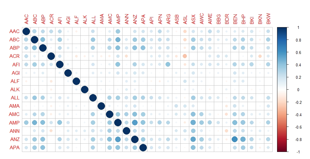
corrplot(correlation_matrix[1:15,1:30])

The above table is a very small part of the full correlation coefficient matrix. Green means positive correlation and red means negative correlation. The diagonal represents the correlation coefficient of a stock with itself so it has all big blue circle of value 1. We are mostly interested in other relation. For example, if we look at the row of ANZ, it has 2 big positive correlation with AMP and BEN which are all not surprisingly in the banking sector. An example of negative correlation is between ACR and ASL which are in different sector. Overall, the negative correlation is rare and could be an option to diversify the investing portfolio.

Correlation coefficient of stocks on 1-day difference

In this section, we look at the correlation coefficient of stocks between 2 business days. We try to figure out if there is any linear relation between stock price today and the stock price tomorrow. The whole process is almost the same except a small twist in how to calculate changedPriceData matrix.

Calculate the correlation matrix.

correlation_matrix_1delay <- matrix(data=NA,nrow=441,ncol=441)
for(i in 1:441)
{
  for(j in 1:441)
  {
    correlation_matrix[i,j]<- a[i,j]=cor(changedPriceData[i,1:563],changedPriceData[j,2:564],use = "complete.obs")}}
  }
}

Visualize the correlation matrix.

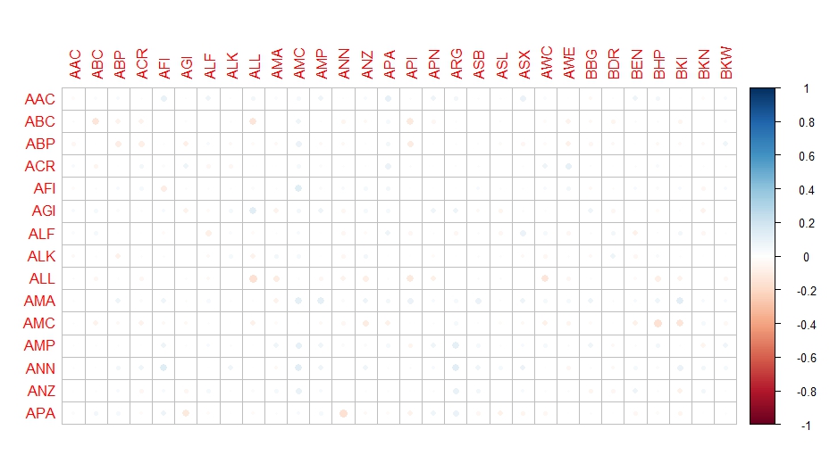
Just by looking at this table, we can say with high certainty that there is no linear relation of stock price over the next business day.