Illion Analytic Exercise
[Machine-Learning Python You have been given a file containing information on a number of loan applicants. Take the provided data set and attempt to identify what factors are useful in predicting loan performance. Report back on your findings, including any issues/concerns with the data.
Summary
Best machine learning model: Decision tree.
Model accuracy: 76.0%
Model precision: 98.5%
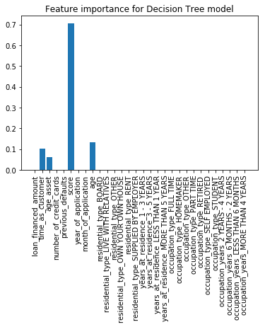
Feature importance (from high to low): Score, age, time as customer, and age asset.
Issues with the data:
- Imbalanced data. After cleaning, BAD loan records are only 4.25% (74/1740) of the whole data set.
- Many missing and inconsistent data entries.
- Some unreliable score values (negative values).
Data overview
The data has 3923 rows and 15 columns originally. A sample is as follow
  date_of_application date_of_birth  loan_financed_amount assessment_outcome  \
0          22/12/2014           NaN               5349.0            Approved
1          11/12/2014           NaN              23350.0            Approved
2           9/01/2015           NaN              10497.0            Approved
3           5/12/2014     18-Jul-48               2920.0                 NaN
4           9/12/2014     22-Jan-70              19466.0            Approved
5           5/12/2014      5-Jan-68              25350.0                 NaN
6           5/12/2014     13-Dec-79              18850.0                 NaN
7          15/12/2014     19-Aug-73              36240.0            Approved
8           7/12/2014     13-Nov-67              29240.0                 NaN
9           8/12/2014     28-Aug-70              35750.0                 NaN

   time_as_customer age_asset   residential_type years_at_residence  \
0             130.0       New                NaN                NaN
1              28.0       New                NaN                NaN
2              27.0       New                NaN                NaN
3               NaN       New               RENT   LESS THAN 1 YEAR
4              41.0       New                NaN                NaN
5               NaN        8+  OWN YOUR OWN HOME        1 - 3 YEARS
6               NaN       New  OWN YOUR OWN HOME        1 - 3 YEARS
7              28.0       New              BOARD        1 - 3 YEARS
8               NaN       New  OWN YOUR OWN HOME  MORE THAN 5 YEARS
9               NaN       New               RENT        1 - 3 YEARS

   number_of_credit_cards         occupation occupation_type  \
0                  0.0                   NaN             NaN
1                  0.0                   NaN             NaN
2                  0.0                   NaN             NaN
3                  NaN               RETIRED         RETIRED
4                  1.0                   NaN             NaN
5                  NaN               ADVISOR       FULL TIME
6                  NaN            TECHNICIAN       FULL TIME
7                  0.0     CUSTOMER SERVICES       FULL TIME
8                  NaN      TICKET INSPECTOR       FULL TIME
9                  NaN              LABOURER       FULL TIME

     occupation_years  previous_defaults  score loan_performance
0                 NaN                  0    519             GOOD
1                 NaN                  0    650             GOOD
2                 NaN                  0    648             GOOD
3   MORE THAN 4 YEARS                  0    715              NaN
4                 NaN                  0    717             GOOD
5   MORE THAN 4 YEARS                  0    777              NaN
6  6 MONTHS - 2 YEARS                  0    682              NaN
7   2 YEARS - 4 YEARS                  0    561              BAD
8   MORE THAN 4 YEARS                  1    523              NaN
9   2 YEARS - 4 YEARS                  0    576              NaN
From the data, we would like to predict the loan performance to be either GOOD or BAD.
The Question
Maximize model precision.
From the data, the majority of loan performance is GOOD and there is only a very small portion of loan performance is actually BAD. Thus, correctly identifying the BAD loans is much more valuable than the GOOD loans. In practice, if a loan application is labeled as BAD, the application would not be proceeded, thus the lender would neither lose or gain money regardless on the prediction accuracy. However, if a loan application is predicted to be GOOD but turns out to be BAD, the lender would lose the lending money, so we want to eliminate this case. In other words, we want to maximize the probability that when a loan is predicted to be GOOD, its performance is actually GOOD. The technical term for this probability is precision. Hence, we will maximize the model precision in later analysis.
Data Preparation
Remove irrelevant columns
‘Occupation’ should not be a factor to determine loan performance. Other reason is that this column has too many non-numeric values so it is not useful for our model anyway.
‘Assessment outcome’ column has only 1 value ‘Approved’ or missing data. Thus, it will not provide any additional information to our model.
import numpy as np
import pandas as pd
import matplotlib.pyplot as plt
import collections
import sklearn
from sklearn.model_selection import train_test_split
from sklearn.tree import DecisionTreeClassifier
from sklearn.ensemble import RandomForestClassifier
from sklearn.linear_model import LogisticRegression
from sklearn.svm import SVC
from sklearn import neighbors
from sklearn.naive_bayes import GaussianNB
import pydotplus

# Set random seed
np.random.seed(1)

#Pandas options
pd.set_option('display.max_rows',200)
pd.set_option('display.max_columns',20)
pd.set_option('display.max_colwidth',20)

data_frame = pd.read_csv('TestData.csv')

#Drop irrelevant columns
data_frame=data_frame.drop(['assessment_outcome','occupation'],axis=1)
Drop missing data entry
#Drop missing data entry
data_frame.dropna(inplace=True)
Drop negative score
Negative scores may be legit and have some meanings. However, due to lack of explaination we do not include negative score in our analysis.
data_frame=data_frame[data_frame['score']>=0]
Convert time
Extract the following information as new columns: ‘age of applicant’, ‘year of application’, ‘month of application’.
#Convert date_of_application and date_of_birth into datetime
new_column=pd.to_datetime(data_frame['date_of_application'])
data_frame['date_of_application']=new_column
new_column=pd.to_datetime(data_frame['date_of_birth'])
data_frame['date_of_birth']=new_column

#Add year_of_application, month_of_application, and age into the data_frame
data_frame['year_of_application']=pd.DatetimeIndex(data_frame['date_of_application']).year
data_frame['month_of_application']=pd.DatetimeIndex(data_frame['date_of_application']).month
data_frame['year_of_birth']=pd.DatetimeIndex(data_frame['date_of_birth']).year
data_frame.loc[data_frame['year_of_birth']>2017,'year_of_birth']-=100
data_frame['age']=(2017 - data_frame['year_of_birth'])

#Drop redundance date_of_application, date_of_birth, year_of_birth
data_frame=data_frame.drop(['date_of_application', 'date_of_birth', 'year_of_birth'],axis=1)
Convert ‘age_asset’ to integer, remove the ‘+’ sign
#Convert age_asset to integer, remove the '+' sign
data_frame.loc[data_frame['age_asset']=='New','age_asset']='0'
data_frame['age_asset'].replace(regex=True,inplace=True,to_replace='\+',value='')
data_frame['age_asset']=pd.to_numeric(data_frame['age_asset'],errors='coerce')
Fix inconsistent data type
#Fix typo in data entry

#data_frame['residential_type'].unique()
#Out[173]:
#array(['BOARD', 'OWN YOUR OWN HOME', 'RENT', 'SUPPLIED BY EMPLOYER',
#       'LIVE WITH RELATIVES', 'OTHER', 'OWN', 'OWN YOUR OWN HOUSE'],
#      dtype=object)
data_frame['residential_type'].replace(inplace=True,to_replace=['OWN','OWN YOUR OWN HOME'],value='OWN YOUR OWN HOUSE')

#data_frame['years_at_residence'].unique()
#Out[177]:
#array(['1 - 3 YEARS', 'MORE THAN 5 YEARS', 'LESS THAN 1 YEAR',
#       '3 - 5 YEARS', '1', '4', '3 YEARS', '5 YEARS OR MORE',
#       '1 - 2 YEARS', '1 YEAR', 'OVER 4 YEARS', 'OVER 1 YEAR',
#       'LESS THAN ONE YEAR', '1 YEAR OR MORE', '5 YEARS OR OVER',
#       '1-3 YEARS', '3-5  YEARS', '3-5 YEARS'], dtype=object)
data_frame['years_at_residence'].replace(inplace=True,to_replace=['5 YEARS OR MORE','5 YEARS OR OVER'],value='MORE THAN 5 YEARS')
data_frame['years_at_residence'].replace(inplace=True,to_replace=['3 YEARS','OVER 4 YEARS','3-5  YEARS','3-5 YEARS','4'],value='3 - 5 YEARS')
data_frame['years_at_residence'].replace(inplace=True,to_replace=['1','1 - 2 YEARS','1 YEAR','OVER 1 YEAR','1 YEAR OR MORE','1-3 YEARS'],value='1 - 3 YEARS')
data_frame['years_at_residence'].replace(inplace=True,to_replace=['LESS THAN ONE YEAR'],value='LESS THAN 1 YEAR')

#data_frame['occupation_type'].unique()
#Out[180]:
#array(['FULL TIME', 'RETIRED', 'SELF EMPLOYED', 'PART TIME', 'OTHER',
#       'HOMEMAKER', 'STUDENT', 'FULLTIME', 'FULL'], dtype=object)
data_frame['occupation_type'].replace(inplace=True,to_replace=['FULLTIME','FULL'],value='FULL TIME')

#data_frame['occupation_years'].unique()
#Out[181]:
#array(['2 YEARS - 4 YEARS', 'MORE THAN 4 YEARS', 'LESS THAN 6 MONTHS',
#       '6 MONTHS - 2 YEARS', '2 - 4 YEARS', '3 YEARS', '2 YEARS',
#       '5 YEARS', '1 YEAR', 'OVER 4 YEARS', 'LESS THAN 1 YEAR',
#       '1 YEAR OR OVER', '1 YEAR OR MORE', '5 YEARS OR MORE',
#       '6 MOTHNS - 2 YEARS', 'LESS THEN 6 MONTHS'], dtype=object)
data_frame['occupation_years'].replace(inplace=True,to_replace=['5 YEARS','OVER 4 YEARS','5 YEARS OR MORE'],value='MORE THAN 4 YEARS')
data_frame['occupation_years'].replace(inplace=True,to_replace=['2 - 4 YEARS','3 YEARS','2 YEARS'],value='2 YEARS - 4 YEARS')
data_frame['occupation_years'].replace(inplace=True,to_replace=['1 YEAR','LESS THAN 1 YEAR','1 YEAR OR OVER','1 YEAR OR MORE','6 MOTHNS - 2 YEARS'],value='6 MONTHS - 2 YEARS')
data_frame['occupation_years'].replace(inplace=True,to_replace=['LESS THEN 6 MONTHS'],value='LESS THAN 6 MONTHS')
Convert non-numeric data into binary
#One-hot encode data
labels=data_frame['loan_performance']
data_frame=data_frame.drop('loan_performance',axis=1)
data_frame=pd.get_dummies(data_frame)
data_frame['loan_performance']=labels
Data Visualization
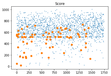
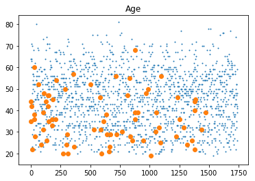
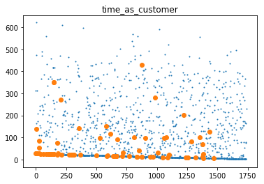
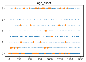
We scatterplot ‘score’, ‘age’, ‘time as customer’, ‘age asset’. The big dots are BAD loans and the small dots are GOOD loans.
# Visualize data
length=len(data_frame['score'])
mask=data_frame['loan_performance']=='GOOD'
good_index=[]
bad_index=[]
for i in range(len(mask)):
    if mask.iloc[i]==True:
        good_index.append(i)
    else:
        bad_index.append(i)

plt.scatter(good_index,data_frame['score'].loc[mask],s=1,label='GOOD')
plt.scatter(bad_index,data_frame['score'].loc[~mask],label='BAD')
plt.title('Score')
plt.show()

plt.scatter(good_index,data_frame['age'].loc[mask],s=1,label='GOOD')
plt.scatter(bad_index,data_frame['age'].loc[~mask],label='BAD')
plt.title('Age')
plt.show()

plt.scatter(good_index,data_frame['time_as_customer'].loc[mask],s=1,label='GOOD')
plt.scatter(bad_index,data_frame['time_as_customer'].loc[~mask],label='BAD')
plt.title('time_as_customer')
plt.show()

plt.scatter(good_index,data_frame['age_asset'].loc[mask],s=1,label='GOOD')
plt.scatter(bad_index,data_frame['age_asset'].loc[~mask],label='BAD')
plt.title('age_asset')
plt.show()
Dealing with Imbalanced Data - Up Sampling
Machine learning models need the number of data points in each class to be roughly in the same size in order to work properly. Otherwise, they will likely treat BAD loans as noise. One simple way to work around the problem is up sampling the minority data. It means replicating BAD loan data so that the number of BAD loan data is closely equal to the number of GOOD loan data.
First, we need to split the data into training set and testing set.
#Split the dataframe into train_frame and test_frame
mask=np.random.rand(len(data_frame))<0.75
train_frame=data_frame[mask]
test_frame=data_frame[~mask]
The training data will be up sampling to train our models. However the testing data will be kept intact and only be used for testing.
#Resampling bad loan data to balance the data classes between good and bad performance
bad_loan_data=train_frame[train_frame['loan_performance']=='BAD']
train_frame=train_frame.append([bad_loan_data]*10,ignore_index=True)

train_labels=train_frame['loan_performance']
train_features=train_frame.drop(['loan_performance'],axis=1)

test_labels=test_frame['loan_performance']
test_features=test_frame.drop(['loan_performance'],axis=1)
Now we are ready to train our models
Baseline Performance
Our baseline model assumes all application is GOOD. The folowing results are obtained with the baseline model for the data after cleaning:
Accuracy: 95.7% Precision: 95.7%
The main reason for this high performance is we only 74 records of BAD loans in the total of about 1700 records. Nevertheless, we are going to improve the precision number.
Model Training
We apply the training data set to a numbers of classification models including Naive Bays, K-nearest Neiboughs, Logistic Regression, Random Forest, Support Vector Machine, and Decision Tree.
###############################
NAIVE BAYES
Predicted  BAD  GOOD
Actual
BAD          9     8
GOOD        86   359
Model accuracy (probability of right prediction):  0.7965367965367965
Precision (Probability that a loan is actually GOOD after being predicted GOOD):  0.9782016348773842
###############################
K-NEAREST NEIGHBORS
Predicted  BAD  GOOD
Actual
BAD          2    15
GOOD        52   393
Model accuracy (probability of right prediction):  0.854978354978355
Precision (Probability that a loan is actually GOOD after being predicted GOOD):  0.9632352941176471
###############################
SUPPORT VECTOR MACHINE
Predicted  BAD  GOOD
Actual
BAD          5    12
GOOD        65   380
Model accuracy (probability of right prediction):  0.8333333333333334
Precision (Probability that a loan is actually GOOD after being predicted GOOD):  0.9693877551020408
###############################
LOGISTIC REGRESSION
Predicted  BAD  GOOD
Actual
BAD          5    12
GOOD        60   385
Model accuracy (probability of right prediction):  0.8441558441558441
Precision (Probability that a loan is actually GOOD after being predicted GOOD):  0.9697732997481109
###############################
RANDOM FOREST
Predicted  BAD  GOOD
Actual
BAD          1    16
GOOD         7   438
Model accuracy (probability of right prediction):  0.9502164502164502
Precision (Probability that a loan is actually GOOD after being predicted GOOD):  0.9647577092511013
###############################
DECISION TREE
Predicted  BAD  GOOD
Actual
BAD         12     5
GOOD       106   339
Model accuracy (probability of right prediction):  0.7597402597402597
Precision (Probability that a loan is actually GOOD after being predicted GOOD):  0.9854651162790697
##############################################
# NAIVE BAYES
clf = GaussianNB()
# Train the Classifier
clf.fit(train_features, train_labels)
# Use the forest's predict method on the test data
predictions = clf.predict(test_features)
# Print model accuracy and True Positive rate
print('###############################')
print('NAIVE BAYES')
Performance_Report(test_labels, predictions)

##############################################
# K-NEAREST NEIGHBORS
clf = neighbors.KNeighborsClassifier()
# Train the Classifier
clf.fit(train_features, train_labels)
# Use the forest's predict method on the test data
predictions = clf.predict(test_features)
# Print model accuracy and True Positive rate
print('###############################')
print('K-NEAREST NEIGHBORS')
Performance_Report(test_labels, predictions)

##############################################
#SUPPORT VECTOR MACHINE
clf = SVC(kernel='linear')
# Train the Classifier
clf.fit(train_features, train_labels)
# Use the forest's predict method on the test data
predictions = clf.predict(test_features)
# Print model accuracy and True Positive rate
print('###############################')
print('SUPPORT VECTOR MACHINE')
Performance_Report(test_labels, predictions)

##############################################
#LOGISTIC REGRESSION
clf = LogisticRegression(random_state=0)
# Train the Classifier
clf.fit(train_features, train_labels)
# Use the forest's predict method on the test data
predictions = clf.predict(test_features)
# Print model accuracy and True Positive rate
print('###############################')
print('LOGISTIC REGRESSION')
Performance_Report(test_labels, predictions)

##############################################
#RANDOM FOREST
clf = RandomForestClassifier(n_jobs=2, random_state=0)
# Train the Classifier
clf.fit(train_features, train_labels)
# Use the forest's predict method on the test data
predictions = clf.predict(test_features)
# Print model accuracy and True Positive rate
print('###############################')
print('RANDOM FOREST')
Performance_Report(test_labels, predictions)

##############################################
#DECISION TREE
clf = DecisionTreeClassifier(criterion = "entropy", random_state = 100,
 max_depth=3, min_samples_leaf=5)
# Train the Classifier
clf.fit(train_features, train_labels)
# Use the forest's predict method on the test data
predictions = clf.predict(test_features)
# Print model accuracy and True Positive rate
print('###############################')
print('DECISION TREE')
Performance_Report(test_labels, predictions)
Factors that are useful to predict loan performance: score(71%), age(13%), time_as_customer(10%), and age_asset(6%).
Tree Visualization
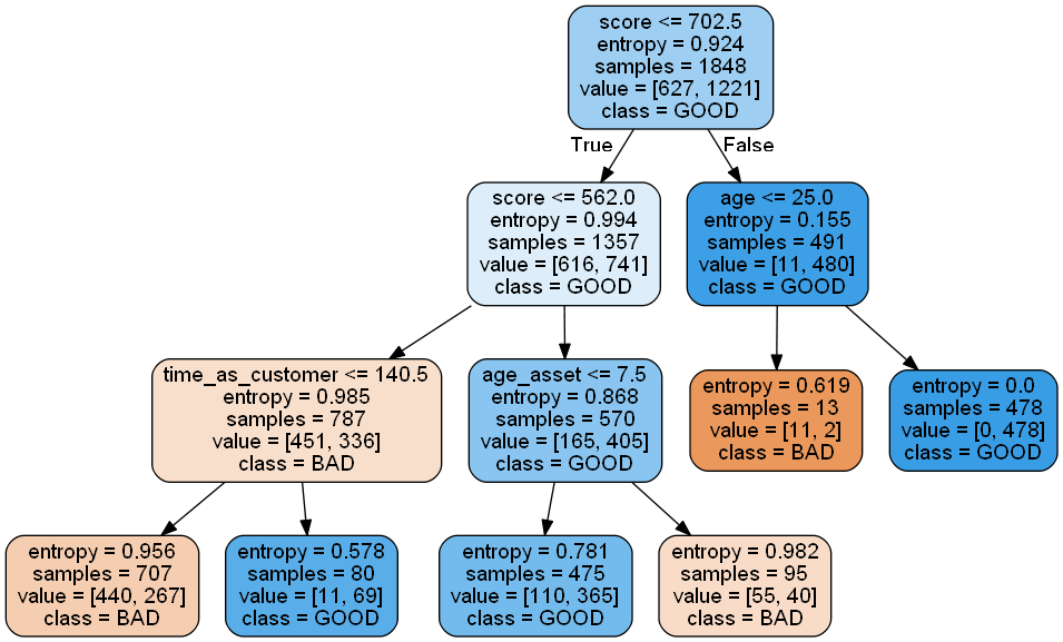
#visualization
data_feature_names = list(train_features)
data_class_names= list(train_labels)
# Visualize data
dot_data = sklearn.tree.export_graphviz(clf,
                                feature_names=data_feature_names,
                                class_names=data_class_names,
                                out_file=None,
                                filled=True,
                                rounded=True)
graph = pydotplus.graph_from_dot_data(dot_data)
graph.write_png('tree.png')
Archive
Machine-Learning Python Matlab Trading Strategy SQL R Algorithm