This project shows how to use linear regression to predict the data trend in Matlab.

The data and business context are extracted from a bigger assignment from the Mahcine Learning course from Coursera at https://www.coursera.org/learn/machine-learning.

Suppose we are running a food truck business which operates over multiple cities. We have some data about the profit of each food truck versus the city population. Then we would like to use those data to predict the profit of a new food truck in a new city. Based on the available data, it is assumed that there is a linear relationship between the city population and profit. We will use linear regression to quantify this relationship.

The data and data visualization

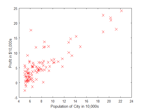
The data source is a csv file with 2 columns where the first column is the city population in 10000s and the second column is the profit in $10000s.

6.1101,17.592
5.5277,9.1302
8.5186,13.662
7.0032,11.854
5.8598,6.8233
8.3829,11.886
7.4764,4.3483
8.5781,12
6.4862,6.5987

Data scatter plot

fprintf('Plotting Data ...\n')
data = load('ex1data1.txt');
X = data(:, 1); y = data(:, 2);
plot(x, y, 'rx', 'MarkerSize', 10); % Plot the data
ylabel('Profit in $10,000s'); % Set the y?axis label
xlabel('Population of City in 10,000s'); % Set the x?axis label

The model and cost function

Suppose we model the relationship between the population and the profit by a linear model as follows

where x_1 is the city population and \theta is our parameter. We would like to optimize the parameter \theta_0 and \theta_1 best fit the model line. It means minimizing the square distance between the actual profit and the hypothesis profit as stated in the following cost function.

where m is the number of data entry. To solve the optimization problem, we may use either gradient descent algorithm or apply the closed form solution. First, we need to calculate the derivative of the cost function.

For gradient descent, each iteration performs the following update.

where \alpha is a positive number which controls how big the jump is in each iteration. Each step the parameter \theta_jcome closer to the optimal values that will achieve the local minimum cost J.

Alternatively, we could calculate \Theta directly based on the closed-form solution as follows.

Solving by gradient descent

The following function calculate the cost J

function J = computeCost(X, y, theta)
%COMPUTECOST Compute cost for linear regression
%   J = COMPUTECOST(X, y, theta) computes the cost of using theta as the
%   parameter for linear regression to fit the data points in X and y
m = length(y); % number of training examples
J = 0;
sum=0;
for i=1:m
   sum=sum+(theta(1)*X(i,1) + theta(2)*X(i,2) - y(i))^2; 
end
J=sum/(2*m);
end

Then use the gradient descent algorithm to find \theta.

function [theta, J_history] = gradientDescent(X, y, theta, alpha, num_iters)
%GRADIENTDESCENT Performs gradient descent to learn theta
%   theta = GRADIENTDESCENT(X, y, theta, alpha, num_iters) updates theta by 
%   taking num_iters gradient steps with learning rate alpha
m = length(y); % number of training examples
J_history = zeros(num_iters, 1);

for iter = 1:num_iters
    temp_theta=theta;
for j=1:length(theta)
    sum=0;
   for i=1:m
       sum=sum+(X(i,1)*theta(1)+X(i,2)*theta(2)-y(i))*X(i,j);
   end
   temp_theta(j)=theta(j)-alpha/m*sum;
end
   theta=temp_theta;
    % Save the cost J in every iteration    
    J_history(iter) = computeCost(X, y, theta);
end
end

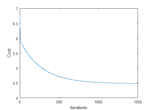
Plot the Cost function over iterations to show convergence.

plot(1:iterations,J_history)
xlabel('Iterations')
ylabel('Cost')

Solving by closed-form solution

It is alot simpler in coding when it comes to closed-form solution.

theta_c=(X'*X)^(-1)*X'*y

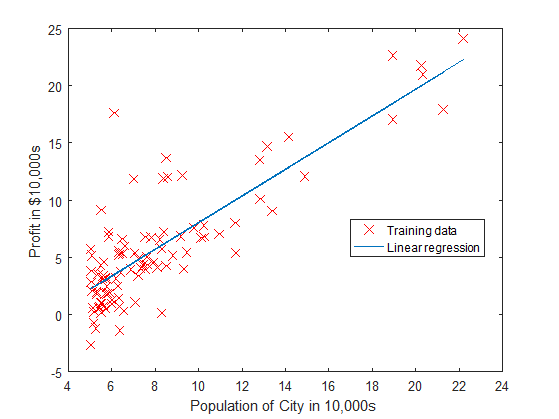
Visualization of the fitting line

hold on; % keep previous plot visible
plot(X(:,2), X*theta, '-')
legend('Training data', 'Linear regression')